A Tutorial on Feature Learning in Shallow Neural Networks
1. Introduction
One of the key drivers behind the success of modern deep learning is the ability of deep neural networks, trained via variants of gradient descent, to learn sophisticated features from data. For example, convolutional networks trained on image data encode both lower-level features such as edges and higher-level features like ears, while language models trained on text corpora can encode features such as semantic information or sentiment. This feature-learning ability is key to the modern paradigm of pretraining and finetuning – pretraining on a large dataset leads to the model learning a diverse set of features, while finetuning extracts the features relevant to that task.
A fundamental question in the quest to build a theory of modern deep learning is to understand precisely how neural networks learn salient features when trained via gradient descent. There are a few challenges with rigorously answering such a question. First, how does one formally define a “feature”? Second, what does it mean for a neural network to “learn” a feature well? Finally, prior toy models such as deep linear networks or kernel methods (as we will see in the next section) fail to capture the notion of complex, nonlinear functions depending on a relevant set of features.
In recent years, progress towards these questions has been made by studying the multi-index model – a simple, solvable model of feature learning in shallow neural networks. Multi-index models are functions which take as input a -dimensional vector, but only depend on an dimensional projection of this input, where is typically much smaller than . Formally, where is the input and is the projection matrix1Each direction in is an “index,” and the function depends on multiple of these directions, hence the name “multi-index”. Multi-index models are a useful proxy for understanding feature learning, as there is a clear notion of a feature: the low-dimensional projection !
The goal of this post is to provide an overview of the main ideas behind learning multi-index models with neural networks. I’ll start by motivating this model as an object of study, summarize the key results and provide intuition for their proofs, and conclude with a discussion of open directions I find particularly exciting.
2. The NTK is unable to capture feature learning
The first generic convergence guarantees for neural networks were based on the neural tangent kernel (NTK) [1] theory. I’ll start with a brief overview of the NTK, and then explain why it falls short when it comes to understanding feature learning. For a detailed discussion of this topic, see Eric Regis’s wonderful blog post.
We are going to let an arbitrary neural network be denoted by , where is the input, are the parameters, and is the function implemented by a neural network with parameters . For instance, if is a two-layer neural network with width , then is the collection of both the first and second layer weights, and the output of the network is defined as The NTK theory posits that a neural network is well-approximated by its first-order Taylor expansion, or linearization, about the initialization. In particular, if are the initial parameters, then the NTK approximation of the neural network is given by While is still a nonlinear function of the input , it is a linear function of the parameters ; indeed, fitting a dataset with is simply a kernel regression problem with fixed feature map .
The key principle behind the NTK theory is that for particular initializations and scaling regimes, the trajectory obtained by running gradient descent on can be coupled to the trajectory obtained by running gradient descent on . In order to prove that gradient descent on converges to a solution with small training error, it suffices to prove the same for the linearized model . But since is linear in the parameters , the loss is convex, which immediately implies convergence to a global minimizer of the training loss! This approach led to some of the first convergence guarantees for gradient descent on a variety of neural network architectures [2,3,4].
However, these NTK-based approaches are missing a key piece of the puzzle of how neural networks are actually trained in practice. Empirically, it has been observed that training a neural network with SGD outperforms training the equivalent NTK [5,6].2This can be due to finite-width effects, large learning rates, minibatch noise, or a variety of other factors. Moreover, the NTK proofs require the approximation in equation (1) to hold throughout the entire training trajectory, which implies that the parameters move very little from their initialization . This NTK regime, or “lazy regime,” refers to a specific choice of initialization and layer scaling where a neural network can interpolate the training data with each neuron moving very little from its initialization [7]. The NTK regime is an undesirable property of neural networks, as ideally some subset of neurons are moving significantly, and the neural network is more than just a kernel method.
These desiderata have motivated muP, or the maximal-update parametrization [8], which is a specific initialization and parametrization scheme which ensures that each neuron has nontrivial movement. muP has also been called the “feature learning” parametrization, where feature learning has been operationalized as neurons moving far from their initialization.3For a pedagogical discussion of muP and its derivation, see Yang et al. [9]. Asymptotic convergence guarantees have been derived for muP [10,11] (or the closely related “mean-field” parametrization, as described in Eric’s post); however, such bounds are either not quantitative (i.e only hold in the limit of infinite width and time) or in the worst case require the network size or training time to grow exponentially in the dimension.
Altogether, we would like to develop a theory of neural network dynamics that captures the feature learning regime. However, we want a definition of feature learning which is stronger than simply requiring that parameters move far from their initialization; we also want to understand how neural networks can recognize underlying structure present in the training data, and utilize this structure to learn quickly.
3. Neural networks are capable of learning features
In order to make progress towards this question, we will posit a specific data-generating process (i.e., a distribution over inputs and a target function ), where the target function depends on some simple features, and analyze the dynamics of neural networks trained on this data distribution.
There are two particular notions of feature learning we will study:
- Mechanistic feature learning: the neural network encodes information about the features within its weights.
- Statistical feature learning: the number of samples needed for a neural network to learn via gradient descent is much smaller than alternate algorithms such as kernel methods, which cannot perform feature learning. We will typically be interested in the asymptotic sample complexity when the input dimension is very large; this ends up being a convenient limit for establishing statistical separations between neural networks and kernel methods4This perspective is common in statistical learning theory and theoretical computer science, where one is typically interested in characterizing the asymptotic sample complexity or runtime as the size of the input grows..
The target function we will focus on is the multi-index model, perhaps the simplest model of feature learning. A multi-index model is a function of the form where is the input, is a low-dimensional projection matrix, and is the link function. The rank is typically assumed to be much smaller than the ambient dimension . A multi-index model has a clear notion of a feature, which is the low-dimensional projection5We will associate the feature with the matrix , the projection , and the subspace spanned by the rows of interchangeably. . If a learner can recognize that the target function only depends on the feature , it is substantially easier for it to learn the rest of the function, which has now reduced to the -dimensional problem of learning .
We will further assume that the input distribution is , the standard isotropic Gaussian in dimensions. This assumes that the input distribution has no underlying structure, and thus all the “feature learning” the network must perform is in recovering . As we will see later, this Gaussian assumption admits a harmonic decomposition and various symmetries that will be convenient for the analyses. See Section 5 for a discussion on moving beyond the Gaussian assumption.
Concretely, we ask the following question.
Consider a dataset of samples generated by and , where is a multi-index model. If a neural network is trained on , how large does need to be to guarantee low test loss?
3.1. The kernel lower bound
The first question we’re interested in is: is feature learning actually needed to learn a multi-index model? While it intuitively makes sense that an algorithm which can extract the low-dimensional representation will obtain a very good sample complexity, could this procedure potentially be implemented with a kernel method like the NTK? The answer to this question turns out to be no: kernel methods require a prohibitively large sample complexity to learn multi-index models.
Theorem 1 [12,13,14], informal. Let be a degree polynomial. Any rotationally invariant kernel method6When the input data is normalized to lie on the unit sphere, a rotationally invariant kernel depends only on the inner product: . This is satisfied for common kernels such as the RBF kernel, or the NTK for isotropic initializations. requires samples to learn the multi-index model .
The space of degree polynomials in dimensions has dimensions (or degrees of freedom), one for each monomial which can be constructed out of the coordinates . Learning an arbitrary polynomial in dimensions would thus require a sample complexity of . Kernel methods are unable to take advantage of the fact that multi-index models have additional low-rank structure, and simply treat them as an arbitrary polynomial, incurring the poor sample complexity. Altogether, this provides a statistical argument demonstrating that kernel methods are unable to perform feature learning.
3.2. Neural networks can learn representations
Neural networks, on the other hand, are capable of learning multi-index models with a significantly improved sample complexity. The key phenomenon behind this sample complexity improvement is the following: the gradient of the loss at initialization reveals the hidden subspace . Below, we will provide some derivations of how exactly the learning dynamics are able to uncover the hidden feature. We emphasize that these derivations will be heuristic, and make a number of simplifying assumptions to help the exposition. We encourage the interested reader to check out the relevant papers for the full, rigorous arguments.
Remark. The goal of this section is to derive end-to-end guarantees for gradient-based learning algorithms. This means we may choose the initialization, learning rates, and other hyperparameters favorably, with the goal of proving that the output of the learning procedure has small loss. This can demonstrate the theoretical power of neural networks in learning various classes of functions. However, the hyperparameter choices here may differ from those made in practice, and proving learning guarantees for “vanilla” gradient descent is an interesting direction of future work; see Section 4.3 for more discussion.
3.2.1. Warmup: single-index model
We will begin by analyzing the dynamics of a neural network trained on a target which is a single-index model, i.e., . In this case, the hidden subspace is simply a vector ; the target function is thus of the form .
Recall that our two-layer neural network is of the form Our objective will be the population (or infinite sample) square loss: Let us compute the gradient of with respect to some neuron . By the chain rule, First, one can show that at initialization, the output of the neural network is close to identically zero.7Under muP or mean field initializations, the second layer weights are mean zero and have standard deviation . Thus for any fixed , the Central Limit Theorem tells us that is a random variable with standard deviation , which converges to once the width is sufficiently large.
Next, we calculate the model gradient: We will additionally make the simplifying assumption that is very small at initialization, and thus . Plugging these both back in, the gradient becomes The gradient at initialization thus points in the direction of the vector .
The key mathematical observation is the following: since the distribution of is rotationally invariant, and depends only on the inner product , the quantity points in the direction of ! To see why, take any vector which is orthogonal to . One then has where the penultimate equality uses the fact that since and are orthogonal, and are independent Gaussians.
![When f(x) = g(<x, u>), the quantity E[x f*(x)] points in the direction of u.](assets/section3_stein_ridge_expectation.png)
When , the quantity points in the direction of .
Lemma 1 (Stein’s Lemma). For any differentiable function ,
Applying Stein’s lemma to gives . Therefore as long as the quantity is nonzero, the gradient points in the direction of the hidden subspace (in this case, the direction ). After one population gradient step, all of the neurons will be pointing in the direction , and thus the neural network will have successfully learned this hidden feature!
3.2.2. A learning guarantee for multi-index models
Let’s now move on to multi-index models. The previous derivation showed that the initial gradient of all neurons pointed in the same direction. For multi-index models, however, there are many hidden directions that must be recovered. We thus must utilize higher-order terms in the expansion of .
Repeating our previous derivation, we can approximate the population gradient by We now Taylor expand8This requires to be twice-differentiable, but Damian et al. [15] generalize this argument to the ReLU activation. to first order to obtain Plugging this in, the loss gradient can be approximated as
This new second term has the effect of rotating each neuron by the matrix . It thus suffices to understand the structure of .
By a similar symmetry argument, since only depends on the projection of onto the subspace spanned by , the matrix must be a low-rank matrix with . Indeed, for any vector with , we have that where the penultimate equality uses the fact that and are independent Gaussians, and the final equality uses the assumption that .
Indeed, two applications of Stein’s Lemma along with the product rule yields:
The matrix thus simplifies as therefore has rank at most ; under the nondegeneracy assumption that is full rank, is exactly a rank matrix whose span coincides with that of . Ignoring the first-order term , since the neurons are initialized randomly, the initial gradients are random vectors lying in the hidden subspace . The initial population gradient step was thus sufficient for recovering the hidden feature , by turning the first layer weights into random vectors in the hidden subspace.
Damian et al. [15] use the above derivation to prove an end-to-end learning guarantee for multi-index models. Formally, they show the following:
Theorem 2 [15]. Let be a multi-index model with rank , and let be a degree polynomial. Assume that ,9This can be achieved by a pre-processing step which fits and then subtracts out the linear component. and has rank . There exists a gradient-based learning algorithm10The learning algorithm is a single gradient step on the first layer with large learning rate, followed by training the second layer with small learning rate until convergence. Dependencies on the width and condition number of are hidden. which with samples obtains a test loss of .
There are a few additional ingredients needed to turn our heuristic derivation into the sample complexity guarantee in Theorem 2:
- The derivation calculates the gradients with respect to the population loss . However, we are actually interested in analyzing gradient descent on the empirical loss over samples . We need to show that, for sufficiently large, the empirical gradients concentrate around their population counterparts. It actually suffices to show that the empirical version of the matrix concentrates close to ; this requires a relatively mild sample complexity of .
- While this shows that the first gradient step can recover the hidden subspace , we’ve still not proven that GD can learn the target with low test error. However, since after the first gradient step the first layer weights are random vectors in the span of , the map is a random feature map restricted to the hidden subspace . It thus suffices to keep fixed and train the second layer weights to convergence. This reduces to a kernel regression problem, but in , rather than dimensions, and thus the sample complexity required to fit to error scales as .
- Error terms from the approximations and equation (3) must be bounded and handled rigorously.
Point 2 above leads to the interesting perspective that neural networks act as an adaptive kernel method; gradient descent learns a subspace on which a kernel method is applied. We’ll discuss this viewpoint further in Section 5.
Altogether, we’ve shown that when the labels are generated by a multi-index model with hidden feature , gradient descent is able to learn this feature by storing the hidden subspace in the first layer weights (our mechanistic notion of feature learning). As a result, neural networks are able to learn multi-index models in samples, significantly fewer than the samples required by kernel methods (our statistical notion of feature learning). This illustrates the adaptivity of neural networks trained via gradient descent: while kernel methods were unable to adapt to the low-dimensionality of , two-layer networks are, and can thus learn much more efficiently.
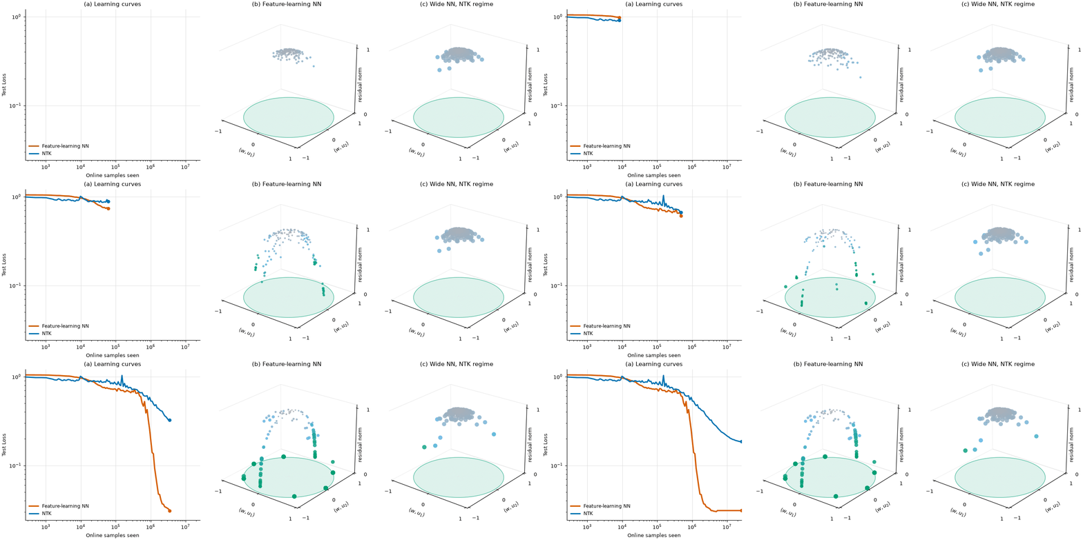
Two layer neural networks trained on a multi-index model with and . (a) Neural networks learn multi-index models in fewer samples than kernel methods (statistical feature learning). (b) Neurons converge to the two-dimensional hidden subspace (mechanistic feature learning). (c) In the NTK regime, most neurons move very little from their initialization.
4. Extensions
4.1. Beyond the non-degeneracy condition: learning hard functions
The learning guarantees in the prior section relied on the non-degeneracy assumption that had rank exactly . There are, however, some natural functions where this condition is violated. Consider the following Gaussian parity function: A simple calculation yields and thus . Is learning still possible in such settings?
Let’s start with the single-index model case, i.e., , for a unit vector . The non-degeneracy assumption then becomes . To understand the complexity of learning in this setting, we’ll need to take a detour into Gaussian space and the Hermite polynomials.
4.1.1. Gaussian space and Hermite polynomials
Since the input distribution is the isotropic Gaussian, it will be natural to work with the function space , the space of square-integrable functions with respect to the Gaussian measure. This is an infinite-dimensional vector space (i.e., a Hilbert space), where the vectors are actually functions . Similar to how inner products and norms are defined on vectors in , we can define inner products and norms between functions as follows: The Hermite polynomials are a sequence of polynomials, where is a degree polynomial, which form an orthonormal basis of . What this means is that, for any , Here are the first few Hermite polynomials:
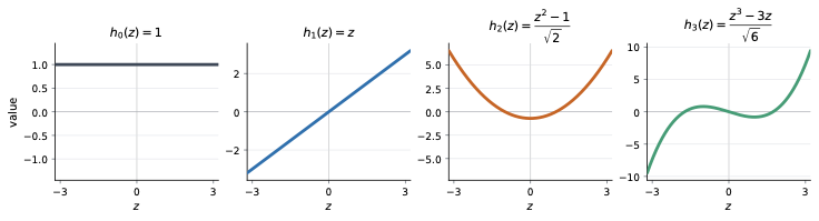
The Hermite polynomials .
Now because the Hermite polynomials form a basis, the link function admits a Hermite decomposition: where the coefficients are the inner products between and the basis functions Analogous to Lemma 1, the can also be expressed in terms of the derivatives of :
The th Hermite polynomial can be interpreted as the degree polynomial which is uncorrelated with all degree polynomials. As such, the coefficient quantifies the size of the “degree component” present in the link function . The non-degeneracy assumptions in Section 3.2 correspond to the terms or being nonzero; in other words, that has a nonzero linear or quadratic component. We can interpret this assumption as requiring there to be sufficient signal in the lower-order terms of which reveal the hidden direction .
4.1.2. The information exponent
Let’s now see what happens to the dynamics when the lower-order terms in equation (4) are zero. We’re going to focus on the case where the learner network is itself a single-index model (equivalently, a neural network with width ): For ease of exposition, we will also assume the target is well-specified: the activation function is equal to the link function .
Let us begin by calculating the population loss for an arbitrary unit vector 11Since we’re restricting to be a unit vector, to make this fully rigorous one needs to analyze the dynamics of spherical gradient descent, where the gradient update gets projected back to the unit sphere. To calculate this expectation, we will utilize another property of Hermite polynomials, which generalizes the orthogonality formula to correlated Gaussians: Applying equation (5), the loss simplifies to and thus the gradient is This population gradient is exactly aligned with the true direction . However, its magnitude depends on the Hermite decomposition of . Since is a fixed unit vector, and is a random unit vector at initialization, the quantity is on the order of . The th term in the gradient scales with , and thus the size of the gradient is dominated by the first nonzero term in the Hermite expansion of . This first nonzero term is called the information exponent [16]:
Definition 1. For a function with Hermite decomposition , the information exponent of is defined as .
The magnitude of the gradient at initialization thus scales as . The information exponent characterizes the geometry of the loss landscape at initialization – a larger information exponent corresponds to a flatter loss landscape near the equator, which increases the difficulty of learning. The finite-sample gradient concentrates at the rate12While scalar averages concentrate at rates, dimensional vectors typically have concentration. , and thus in order for the true gradient signal to overpower the finite-sample noise, one must take , or .
Online SGD. A similar picture holds if one instead considers training via online SGD with a constant batch size. At each time step, the gradient has very little correlation with the true direction , and is dominated by the noise in the current minibatch. The initial stage of SGD is thus a long plateau – the iterate stays close to the equator (i.e stays close to ), while the loss stays near its initial value. Eventually, after very many gradient steps, the iterate manages to escape the equator and rapidly converge to . Arous et al. [16] show that samples13This is a factor of improvement over the sample complexity required to recover in a single step, and is due to a refined martingale concentration technique. (or equivalently time steps) are required to learn a single-index model with information exponent . Moreover, the learning dynamics exhibit a long plateau phase of length , followed by a rapid descent phase of length .
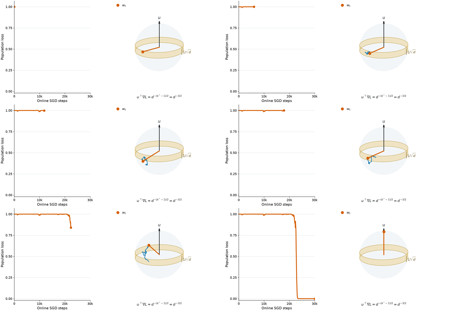
Learning the single-index model via online SGD. The loss curve exhibits a long plateau as the iterate escapes the high-entropy equator, followed by a sharp transition as converges to .
Finally, we remark that while this proof sketch was for the setting where the learner is a single-index model, similar proof techniques hold when the learner is a two-layer ReLU network [17] under a two-stage learning procedure where in the first stage all neurons converge to the direction , and in the second stage the are trained to fit the link function.
4.2. Staircase Functions
For single-index models, the information exponent governs the difficulty of learning the hidden direction via SGD. For multi-index models, however, the picture can become more complicated. When there are multiple directions in the target subspace which must be recovered, some of these may be easy (i.e., have correlation with low-degree polynomials), while others might be hard.
Let’s return to our example Gaussian parity function This is a multi-index model with rank . One can check that is orthogonal to all polynomials of degree 3 or fewer,14It suffices to consider monomials, which can depend on at most 3 of . and as such requires samples to be learned via online SGD.15This is by analogy to the information exponent 4 setting in the prior section, but is made rigorous for multi-index models in Abbe et al. [18].
Let us compare this to the following target, which is called a staircase function: The first-order term, which from Section 3.2.1 is recoverable in samples, is However, at least naively, it is not clear how one can recover the remainder of the directions in the hidden subspace without using far more than samples.
Quite surprisingly, Abbe et al. [18] show that neural networks can utilize the easy directions in order to learn the hard directions in much fewer samples. In particular, once the direction has been learned, the “missing” component of is The first-order term of this missing component is and thus can be recovered in another samples. This procedure proceeds sequentially; once is learned, the network learns , and then finally . The total sample complexity is – far smaller than the sample complexity required to learn the high-degree monomial !
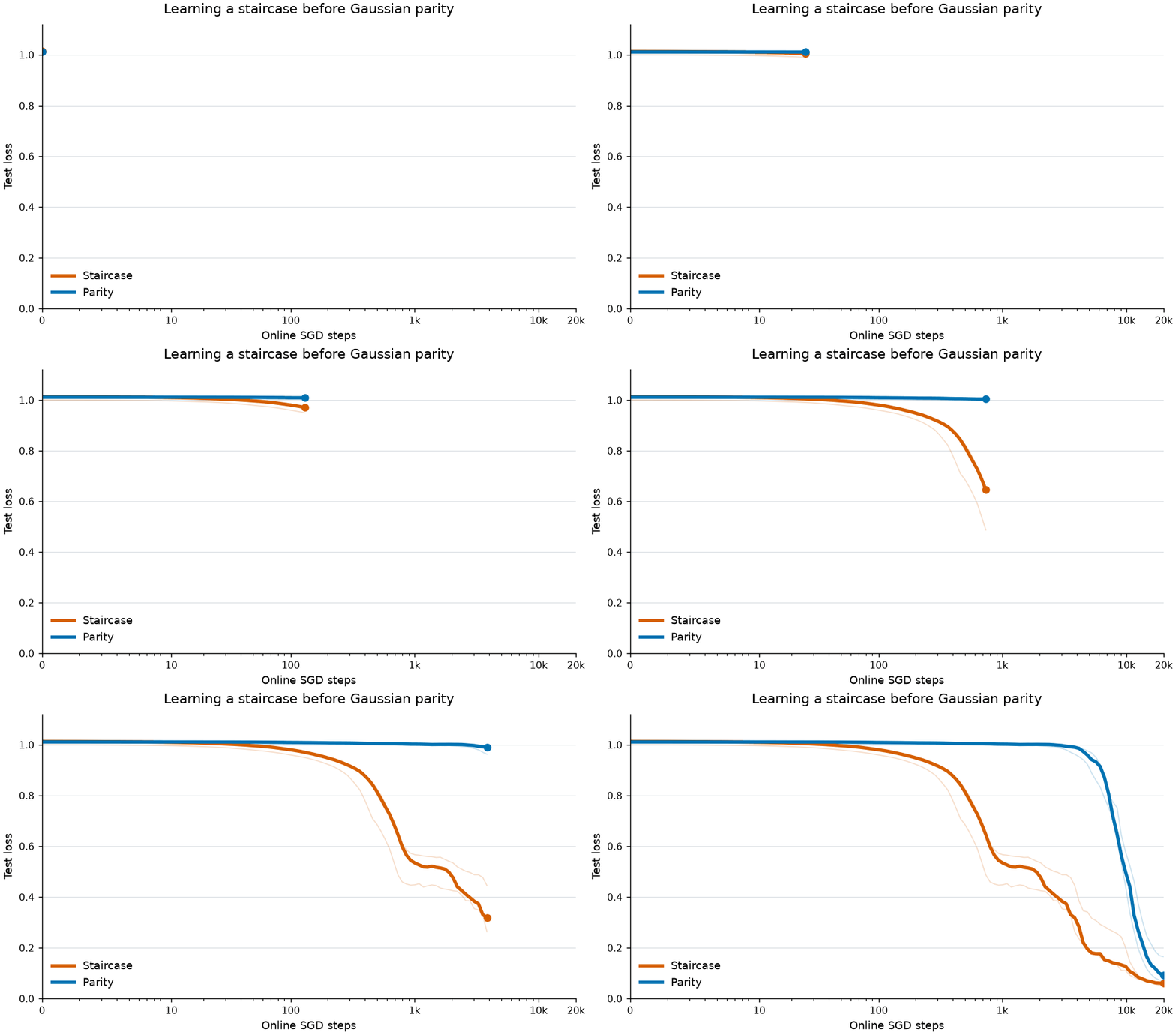
Neural networks can learn the staircase function much more efficiently than the parity function .
The learning dynamics thus proceed as a staircase, with the lower-order terms acting as stepping stones which aid in the learning of the higher-order terms.16See Dandi et al. [19] for a fine-grained characterization of which directions can be learned via multiple steps of GD. This also illustrates the simplest case of how neural networks can learn hierarchical structure – where low order terms aid in the learning of high order terms. See Section 5 for more discussion and open questions on learning hierarchical targets.
Abbe et al. [18] study a more general family of multi-index models, and introduce the leap complexity, which generalizes the information exponent by quantifying the maximum “leap” in degree that must be made in order to learn another direction in the hidden subspace. For example, for sums of monomials of the form where , the size of the th leap is , and the leap complexity is defined as . Abbe et al. [18] show that a variant of SGD17Layerwise training, and dependent on the basis of the staircase. will learn this function by learning each monomial one at a time, and where the th monomial is learned with a sample complexity of . Moreover, from an optimization landscape perspective, the training exhibits a saddle-to-saddle dynamics – the th saddle corresponds to the neural network having learned the first monomials, at which the loss will plateau for a length of time proportional to until the th monomial is learned.
This leap complexity and saddle-to-saddle picture is generalized to arbitrary multi-index models in Bietti et al. [20]. While their analysis is focused on the population gradient-flow and an idealized “two-timescale” learning procedure, they demonstrate how the learning of a multi-index model proceeds through a sequence of saddles corresponding to sequentially learning directions in the hidden subspace, where the time required to escape each saddle scales with its corresponding leap. However, a finite-sample convergence result for learning multi-index models under “standard” training conditions remains open.
4.3. Further Extensions & Generalizations
Boolean data. So far, we have focused on the case where the input distribution is the isotropic Gaussian. A similar picture emerges when the inputs are drawn uniformly from the Boolean hypercube (i.e., each coordinate is sampled independently from ). Here, the canonical hard learning problem is the -sparse parity function. The -sparse parity selects some hidden subset of size , and defines The parameter acts analogously to both the rank (i.e., the size of the sparse subset the target depends on) and the information exponent (the lowest degree polynomial which has nonzero correlation with the target). In order to learn , a neural network must learn to recover the hidden sparse subset .
Barak et al. [21] show that a two-layer neural network with width trained via layerwise SGD can learn the -sparse parity task with a sample complexity of .18Kernel methods also succeed in samples, yet must have a size (i.e., feature dimension) of as well; the advantage of neural networks in the feature learning regime is that they require a significantly smaller width. The learning dynamics follow a similar story as in the multi-index setting – during the first stage, the first layer weights learn to encode the hidden subset , and in the second stage, the second layer weights converge to implement .
The staircase phenomenon described in Section 4.2 holds as well. Abbe et al. [22] show that for Boolean staircase functions of the form SGD gradually learns the support and only needs samples to learn each individual coordinate, thus requiring only total samples to learn the entire target.
Modeling deep learning phenomena. Multi-index models can also act as a useful abstraction for understanding other deep learning phenomena, beyond feature learning. In Section 4.2, we saw that certain multi-index models exhibit saddle-to-saddle dynamics, leading to staircase learning curves. This is analogous to saddle-to-saddle dynamics exhibited in simpler models such as deep linear networks [23,24], and captures the stepwise learning dynamics exhibited by deep neural networks in practice.
Multi-index models have also been used to model the existence of neural scaling laws. As neural networks are scaled up in compute, they exhibit two seemingly contradictory phenomena – individual task performances exhibit sharp transitions, while the overall loss follows a smooth, power-law decay. To reconcile this, Michaud et al. [25] proposed the quantization hypothesis.19See Eric Michaud’s excellent blog post here. This posits that neural network dynamics consist of a sequence of discrete quanta whose learning curves exhibit sharp transitions; however, since there are many such quanta and these phase transitions occur at different timescales, the overall loss follows a smooth, power-law decay. Ren et al. [26] prove that this picture precisely occurs when the target function is itself a two-layer neural network . In Section 4.1.2, we saw that the learning curve for a single-index model exhibited a long plateau followed by a rapid descent. Ren et al. [26] show that for learning the two-layer network, the loss curve for each individual neuron follows a sharp transition at time proportional to ; yet since the overall loss sums over these many neurons, it follows a smooth, power-law decay. The individual neurons are thus precisely the discrete quanta!
Lower bounds and optimal sample complexities. One may ask whether the sample complexity for learning information-exponent functions is optimal. The answer here ends up being no – the information exponent is actually a property of the learning algorithm (here online SGD), while the computational complexity of learning can be quite different. Indeed, modifications to the learning procedure can lead to different characterizations of the difficulty of learning. For example, Damian et al. [27] show that explicitly smoothing the loss landscape (roughly speaking, averaging the loss in the neighborhood of the current parameter) amplifies the gradient signal around random initialization, and leads to learning information-exponent functions with a sample complexity of .
Even more strikingly, a recent line of work [28,29,30] has shown that reusing samples can also significantly improve the sample complexity of recovering the hidden subspace. The analyses we’ve considered so far focus on one-pass SGD, where each gradient step is computed on a fresh batch of data. As such, if the target function has no low-degree term, then SGD is unable to extract any signal. However, if the same data points are used for multiple updates, dependence between iterates can lead to nonlinear transformations of the input, which may then reveal low-degree signal. For the case of polynomials, Lee et al. [30] show that a specific sample-reuse procedure can lead to learning arbitrary single-index polynomials with samples – independent of the information exponent! This suggests a potentially important mechanism for practical gradient descent; however, it remains open to understand whether neural networks under standard training can exploit this mechanism optimally.
Finally, I will remark that there is a rich recent literature on algorithms and lower bounds for learning multi-index models, beyond SGD; the interested reader should consult the survey [31] and the references therein.
5. Open Directions
Let’s take a step back and summarize what we’ve covered so far. Our motivating question was to understand how neural networks trained via SGD can perform feature learning. For the setting of learning Gaussian multi-index models – a stylized model of feature learning where the feature corresponds to the low-dimensional subspace – we showed how two-layer neural networks trained via SGD can learn features with far fewer samples than kernel methods. While a number of interesting mathematical questions remain open,20Namely: deriving end-to-end learning guarantees for generic multi-index models, and understanding the robustness of the batch-reuse phenomenon. the prior works we’ve covered have painted a clear conceptual picture of how feature learning occurs in this simple sandbox.
So where do we go next? The multi-index model was designed to be a stepping stone towards understanding more sophisticated forms of feature learning performed by neural networks in practice. I think that the most interesting future directions involve coming up with new settings and abstractions to analyze these more general feature learning phenomena. Below are a few directions I find particularly exciting:
Beyond Gaussian data. One of the biggest limitations of the prior works is that they assume the input distribution is the isotropic Gaussian (or uniform over the Boolean hypercube). The proofs we’ve covered rely heavily on this rotational invariance assumption, either to argue that the initial gradient step recovers the hidden subspace, or to reduce the SGD dynamics to only analyzing the overlap of each neuron with the hidden feature. Real-world data distributions such as images, however, are far from Gaussian. Some works have aimed to generalize existing single-index model analyses to distributions which are close to Gaussian [32], or non-isotropic Gaussian [33]. Yet real-world data distributions may themselves possess low-dimensional structure, such as lying on a low-dimensional manifold [34]. One interesting question is thus to understand what features neural networks can learn, and at what statistical and computational complexity, when both the input distribution and the target function depend on a low-dimensional feature.
Open Question #1: How do neural networks learn features when both the input distribution and the target function are “low-dimensional”?
Hierarchical feature learning and the role of depth. The multi-index model captures a basic example of feature learning, as once the learner recovers the feature , it is easy for it to learn the remainder of the target function. In practice, however, it is believed that neural networks use depth to learn a hierarchy of features. For example, in image classification, the first layer may detect edges, while the next may use these edge features to detect shapes. Each layer of the neural network is thus learning a progressively more complex feature.
Open Question #2: How do neural networks use depth to learn a hierarchy of features?
Let me summarize initial progress made towards this question. A multi-index model is simply a target function of the form , where the hidden feature is the linear function . By considering more general features – say polynomial functions – one obtains a larger family of hierarchical functions. A recent line of work [35,36,37] has shown that three-layer neural networks are capable of efficiently learning such hierarchical functions for a certain class of polynomial features . The learning dynamics proceed similarly to Section 3.2 – the first layer encodes a random feature map, and a single large gradient step on the second layer is able to recover the feature . Such functions are not learnable via two-layer neural networks, and thus this establishes a separation between the power of two- and three-layer networks from the perspective of learnability via SGD. More generally, [38,39] introduce hierarchical variants of the multi-index model, where each layer in the hierarchy implements a multi-index model of the output of the previous layer. These works demonstrate cases where GD on a deep network can learn this sequence of features and thus the target function with significantly fewer samples than a shallower network.
While the models we’ve discussed so far operate on continuous inputs, natural language is made up of discrete sequences of tokens, yet nonetheless possesses hierarchical structure we may want a neural network to learn. One interesting question is thus to develop simplified theoretical models which capture the hierarchical structure of language, and understand the extent to which neural networks trained via SGD can learn these models. One example is the Random Hierarchy Model (RHM) [40], a generative model for language where the label of each input sequence depends on a hierarchy of progressively higher level features. Ren et al. [41] show that deep convolutional networks trained via GD can efficiently learn an RHM by learning the hierarchy of relevant features. Developing more general models for language, as well as for domains such as formal math or scientific data, and understanding the dynamics of neural networks when trained on such tasks is another exciting future direction.
Open Question #3: What are theoretical models which capture the hierarchical structure of real-world data, and how are they learned by neural networks?
Connections to feature learning in practice. Stylized analyses of feature learning can still provide insight towards how neural networks are trained in practice, and potentially suggest alternate learning procedures. One relevant mechanism is the Neural Feature Ansatz [42], which posits that the features encoded by the th layer of a neural network are the “average gradient outer product” of the model output with respect to the input to that layer. For the first layer of a neural network , the Ansatz reduces to When the target function is a multi-index model, equation (6) implies that the first layer weights will learn the hidden subspace , coinciding with our derivation in Section 3.2.2. Radhakrishnan et al. [42] also introduce the Recursive Feature Machine algorithm, an adaptive kernel method which alternates between estimating a subspace of relevant features and fitting a kernel method to these relevant features. This aligns with what we observed for two-layer neural networks, where the training of the second layer is a kernel regression problem with a learned kernel depending only on the subspace .
Another proposed mechanism, called Neural LoFi [43], takes direct motivation from the multi-index derivation. In two-layer networks, we saw that the learned features were given by the matrix . Dandi et al. [43] define an idealized learning procedure where the “features” learned by the th layer are the top eigenvectors of the matrix , where are the outputs of the previous layer. This procedure agrees with performance of neural networks trained with gradient descent in the early stages of training, learns salient feature maps when trained on image data, and casts hierarchical feature learning in deep networks as a composition of simple, low-degree features.
Open Question #4: What else can our existing stylized analyses of feature learning tell us about how neural networks learn features in practice?
Analyses of vanilla gradient descent. The critical reader may point out that none of the algorithms we’ve discussed correspond to gradient descent literally as it is implemented in practice; indeed, each of these algorithms relies on various “tricks” such as layerwise training or well-chosen initializations and learning rates. Empirically, however, the ability of neural networks to learn multi-index models is much more robust, and occurs beyond just the theoretical settings for which we have provable guarantees. While analyzing stylized variants of SGD provides a starting point towards understanding which behaviors can be learned by neural networks, our ultimate goal is to characterize the learning dynamics under “standard training” conditions such as common initialization schemes and joint training of both layers. Some initial progress has been made towards this goal: Glasgow [44] shows that for the task of learning the XOR (or 2-sparse parity) function , standard training of a two-layer neural network can learn in samples. Deriving similar learning guarantees for more general families of multi-index models remains an interesting open question, and may require fundamentally new techniques.
Open Question #5: Can we analyze the dynamics of gradient descent under “standard” training assumptions?
References
- Arthur Jacot, Franck Gabriel, and Clément Hongler. Neural tangent kernel: Convergence and generalization in neural networks. NeurIPS, 2018.
- Mahdi Soltanolkotabi, Adel Javanmard, and Jason D. Lee. Theoretical insights into the optimization landscape of over-parameterized shallow neural networks. IEEE Transactions on Information Theory, 2018.
- Simon S. Du, Xiyu Zhai, Barnabas Poczos, and Aarti Singh. Gradient descent provably optimizes over-parameterized neural networks. arXiv:1810.02054, 2018.
- Simon Du, Jason Lee, Haochuan Li, Liwei Wang, and Xiyu Zhai. Gradient descent finds global minima of deep neural networks. ICML, 2019.
- Sanjeev Arora, Simon S. Du, Wei Hu, Zhiyuan Li, Russ R. Salakhutdinov, and Ruosong Wang. On exact computation with an infinitely wide neural net. NeurIPS, 2019.
- Jaehoon Lee, Samuel Schoenholz, Jeffrey Pennington, Ben Adlam, Lechao Xiao, Roman Novak, and Jascha Sohl-Dickstein. Finite versus infinite neural networks: an empirical study. NeurIPS, 2020.
- Lenaic Chizat, Edouard Oyallon, and Francis Bach. On lazy training in differentiable programming. NeurIPS, 2019.
- Greg Yang and Edward J. Hu. Tensor Programs IV: Feature learning in infinite-width neural networks. ICML, 2021.
- Greg Yang, James B. Simon, and Jeremy Bernstein. A spectral condition for feature learning. arXiv:2310.17813, 2023.
- Song Mei, Andrea Montanari, and Phan-Minh Nguyen. A mean field view of the landscape of two-layers neural networks. Proceedings of the National Academy of Sciences 115.33 (2018): E7665-E7671.
- Lenaic Chizat and Francis Bach. On the global convergence of gradient descent for over-parameterized models using optimal transport. NeurIPS, 2018.
- Behrooz Ghorbani, Song Mei, Theodor Misiakiewicz, and Andrea Montanari. Limitations of lazy training of two-layers neural network. NeurIPS, 2019.
- Behrooz Ghorbani, Song Mei, Theodor Misiakiewicz, and Andrea Montanari. Linearized two-layers neural networks in high dimension. 2021.
- Daniel Hsu. Dimension lower bounds for linear approaches to function approximation. arXiv:2508.13346, 2025.
- Alexandru Damian, Jason Lee, and Mahdi Soltanolkotabi. Neural networks can learn representations with gradient descent. COLT, 2022.
- Gerard Ben Arous, Reza Gheissari, and Aukosh Jagannath. Online stochastic gradient descent on non-convex losses from high-dimensional inference. JMLR, 2021.
- Alberto Bietti, Joan Bruna, Clayton Sanford, and Min Jae Song. Learning single-index models with shallow neural networks. NeurIPS, 2022.
- Emmanuel Abbe, Enric Boix Adsera, and Theodor Misiakiewicz. SGD learning on neural networks: leap complexity and saddle-to-saddle dynamics. COLT, 2023.
- Yatin Dandi, Florent Krzakala, Bruno Loureiro, Luca Pesce, and Ludovic Stephan. How two-layer neural networks learn, one (giant) step at a time. JMLR, 2024.
- Alberto Bietti, Joan Bruna, and Loucas Pillaud-Vivien. On learning Gaussian multi-index models with gradient flow part I: General properties and two-timescale learning. Communications on Pure and Applied Mathematics, 2025.
- Emmanuel Abbe, Enric Boix Adsera, and Theodor Misiakiewicz. The merged-staircase property: a necessary and nearly sufficient condition for SGD learning of sparse functions on two-layer neural networks. COLT, 2022.
- Arthur Jacot, François Ged, Berfin Şimşek, Clément Hongler, and Franck Gabriel. Saddle-to-saddle dynamics in deep linear networks: Small initialization training, symmetry, and sparsity. arXiv:2106.15933, 2021.
- Scott Pesme and Nicolas Flammarion. Saddle-to-saddle dynamics in diagonal linear networks. NeurIPS, 2023.
- Eric Michaud, Ziming Liu, Uzay Girit, and Max Tegmark. The quantization model of neural scaling. NeurIPS, 2023.
- Yunwei Ren, Eshaan Nichani, Denny Wu, and Jason Lee. Emergence and scaling laws in SGD learning of shallow neural networks. NeurIPS, 2025.
- Alex Damian, Eshaan Nichani, Rong Ge, and Jason D. Lee. Smoothing the landscape boosts the signal for SGD: Optimal sample complexity for learning single index models. NeurIPS, 2023.
- Yatin Dandi, Emanuele Troiani, Luca Arnaboldi, Luca Pesce, Lenka Zdeborová, and Florent Krzakala. The benefits of reusing batches for gradient descent in two-layer networks: Breaking the curse of information and leap exponents. arXiv:2402.03220, 2024.
- Luca Arnaboldi, Yatin Dandi, Florent Krzakala, Luca Pesce, and Ludovic Stephan. Repetita iuvant: Data repetition allows SGD to learn high-dimensional multi-index functions. arXiv:2405.15459, 2024.
- Jason D. Lee, Kazusato Oko, Taiji Suzuki, and Denny Wu. Neural network learns low-dimensional polynomials with SGD near the information-theoretic limit. NeurIPS, 2024.
- Joan Bruna and Daniel Hsu. Survey on algorithms for multi-index models. Statistical Science, 2025.
- Aaron Zweig, Loucas Pillaud-Vivien, and Joan Bruna. On single-index models beyond Gaussian data. NeurIPS, 2023.
- Alireza Mousavi-Hosseini, Denny Wu, Taiji Suzuki, and Murat A. Erdogdu. Gradient-based feature learning under structured data. NeurIPS, 2023.
- Mikhail Belkin and Partha Niyogi. Laplacian eigenmaps for dimensionality reduction and data representation. Neural Computation, 2003.
- Eshaan Nichani, Alex Damian, and Jason D. Lee. Provable guarantees for nonlinear feature learning in three-layer neural networks. NeurIPS, 2023.
- Zihao Wang, Eshaan Nichani, and Jason Lee. Learning hierarchical polynomials with three-layer neural networks. ICLR, 2024.
- Hengyu Fu, Zihao Wang, Eshaan Nichani, and Jason Lee. Learning hierarchical polynomials of multiple nonlinear features. ICLR, 2025.
- Yatin Dandi, Luca Pesce, Lenka Zdeborová, and Florent Krzakala. The computational advantage of depth in learning high-dimensional hierarchical targets. NeurIPS, 2025.
- Joan Bruna. The multiscale single-index model: A stylized model for hierarchical feature learning. arXiv:2607.03347, 2026.
- Francesco Cagnetta, Leonardo Petrini, Umberto M. Tomasini, Alessandro Favero, and Matthieu Wyart. How deep neural networks learn compositional data: The random hierarchy model. Physical Review X, 2024.
- Yunwei Ren, Yatin Dandi, Florent Krzakala, and Jason D. Lee. Provable learning of random hierarchy models and hierarchical shallow-to-deep chaining. arXiv:2601.19756, 2026.
- Adityanarayanan Radhakrishnan, Daniel Beaglehole, Parthe Pandit, and Mikhail Belkin. Mechanism for feature learning in neural networks and backpropagation-free machine learning models. Science, 2024.
- Yatin Dandi, Matteo Vilucchio, Luca Arnaboldi, Hugo Tabanelli, and Florent Krzakala. Deep learning as neural low-degree filtering: A spectral theory of hierarchical feature learning. arXiv:2605.13612, 2026.
- Margalit Glasgow. SGD finds then tunes features in two-layer neural networks with near-optimal sample complexity: A case study in the XOR problem. ICLR, 2024.